I’ve written before about plots that are more informative than your standard barplot.
Another option is the joyplot (also known as frequency trails). Joyplots are like mountain ranges, except instead of mountains it’s smoothed density histograms. It’s a way to visualize a lot of data in a pretty compact space.
Claus Wilke has written an R package that makes plotting these pretty frictionless. Just add data!
I’ll whip up some fake data to play with.
set.seed(123)
joy <- data.frame('label'=rep(letters[1:10], each=100),
                  'value'=as.vector(mapply(rnorm, rep(100, 10), rnorm(10), SIMPLIFY=TRUE)),
                  'rank'=rep(1:5, each=100, times=20))
Here’s an example in which the distributions are allowed to overlap vertically, giving the appearance that they are stacked.
suppressPackageStartupMessages({
  library(ggjoy)
  library(dplyr)
  library(ggplot2)})

ggplot(joy, aes(x=value, y=label)) +
  geom_joy(scale=2, rel_min_height=.03) +
  scale_y_discrete(expand = c(0.01, 0)) +
  xlab('Value') +
  theme_joy() +
  theme(axis.title.y = element_blank())
## Picking joint bandwidth of 0.209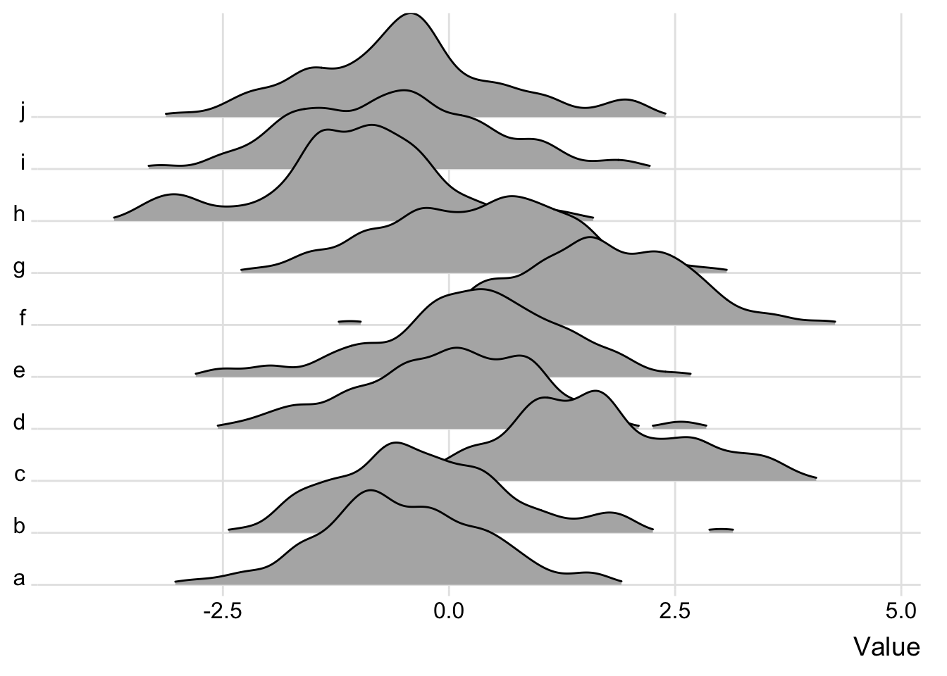 To make things look more orderly, and since our labels have no inherent order, we can order the data according to the mean. This isn’t neccessary if your y-axis is time, for instance.
joy <- group_by(joy, label) %>%
       mutate(m=mean(value)) %>%
       arrange(m) %>%
       ungroup() %>%
       mutate(label=factor(label, unique(label)))

ggplot(joy, aes(x=value, y=label)) +
  geom_joy(scale=2, rel_min_height=.03) +
  scale_y_discrete(expand = c(0.01, 0)) +
  xlab('Value') +
  theme_joy() +
  theme(axis.title.y = element_blank())
## Picking joint bandwidth of 0.209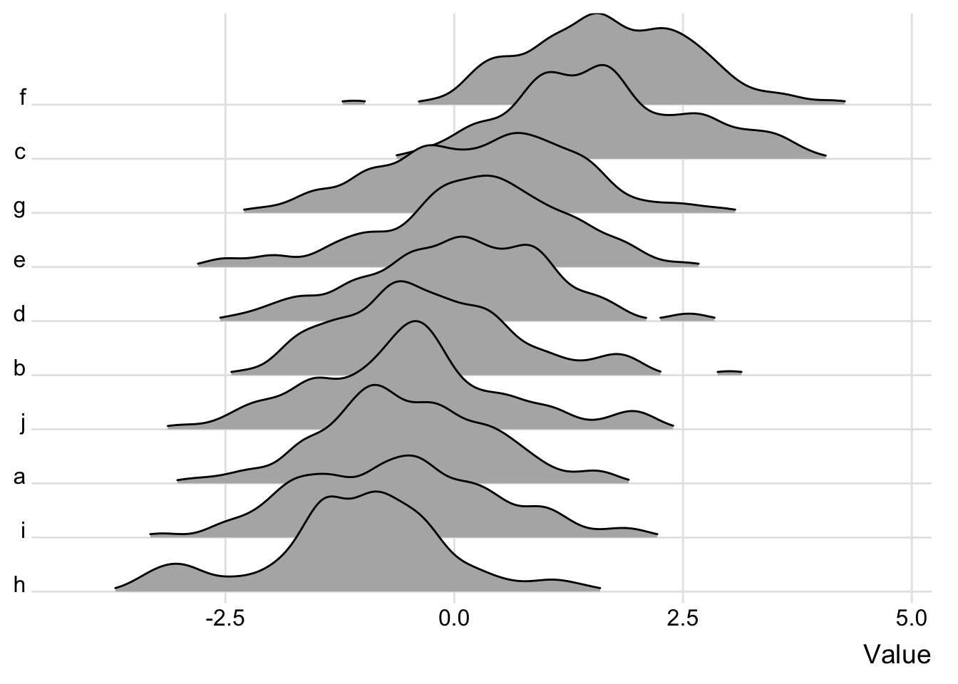
Some people don’t like this overlap (for the aesthetics or because it can obscure the data) so here’s an example if we spread everybody out so that they don’t touch. The amount of overlap is easily controlled by the scale argument in geom_joy. scale = 1 means no overlap; the higher this value, the more the distributions will overlap.
ggplot(joy, aes(x=value, y=label)) +
  geom_joy(scale=1, rel_min_height=.01) +
  scale_y_discrete(expand = c(0.001, 0)) +
  xlab('Value') +
  theme_joy() +
  theme(axis.title.y = element_blank())
## Picking joint bandwidth of 0.209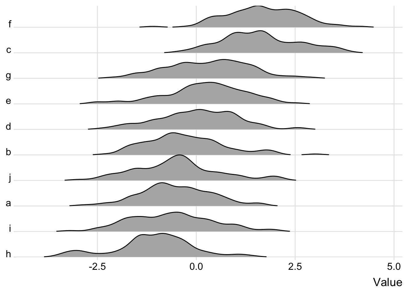
How about some color? Color can be used to separate groups:
ggplot(joy, aes(x=value, y=label, fill=as.factor(rank))) +
  geom_joy(scale=1, rel_min_height=.01) +
  scale_y_discrete(expand = c(0.01, 0)) +
  xlab('Value') +
  labs(fill='Rank') +
  theme_joy() +
  theme(axis.title.y = element_blank())
## Picking joint bandwidth of 0.209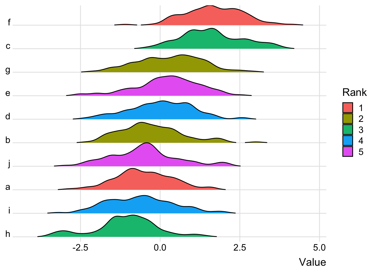
Or, if your data doesn’t have grouping structure, it can just be used to break things up a little bit. (See this tweet for another example.)
ggplot(joy, aes(x=value, y=label, fill=label)) +
  geom_joy(scale=3, rel_min_height=0.01) +
  scale_fill_manual(values=rep(c('gray', 'lightblue'), length(unique(joy$label))/2)) +
  scale_y_discrete(expand = c(0.01, 0)) +
  xlab('Value') +
  theme_joy() +
  theme(axis.title.y = element_blank(),
        legend.position='none')
## Picking joint bandwidth of 0.209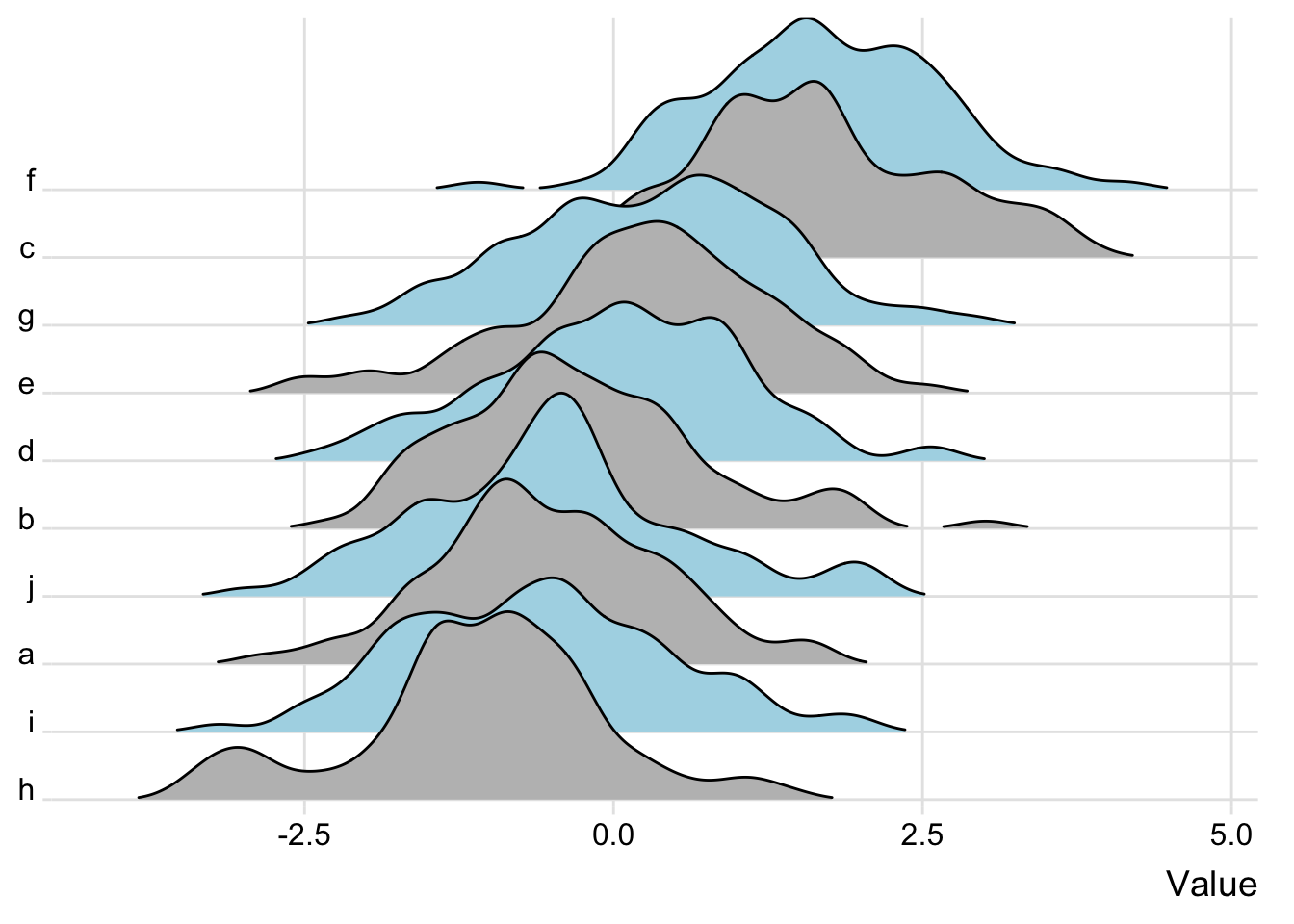
How about some joyful facets?
ggplot(filter(joy, rank != 5), aes(x=value, y=label)) +
  geom_joy(scale=1, rel_min_height=.03) +
  scale_y_discrete(expand = c(0.01, 0)) +
  xlab('Value') +
  facet_wrap(~rank, scales='free') +
  theme_joy() +
  theme(axis.title.y = element_blank())
## Picking joint bandwidth of 0.202## Picking joint bandwidth of 0.219## Picking joint bandwidth of 0.198## Picking joint bandwidth of 0.229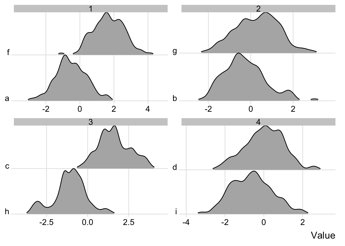
You can check out the vignette for more examples and more information. You can also check out the docs for information on, for example, how the density is calculated and what your options are for that.
If you want to play around with these yourself, you can make up data (like I did) or check out the examples in the vignette for datasets to use that will make cool plots. Who knows–you might even find the iris dataset fun again if you use it to make joyplots.