Intro to Bootstrapping

The bootstrap, detailed by Efron and Tibshirani in their 1993 book An Introduction to the Bootstrap, is a powerful, flexible statistical concept based on the idea of “pulling yourself up by your bootstraps.” With today’s computing power, it’s easier than ever to apply and use. It also happens to be one of my favorite statistical tricks because of the elegance of the underlying logic.

The idea behind the bootstrap is simple. We know that if we repeatedly sample groups from the population, our measurement of that population will get increasingly accurate, becoming perfect when we’ve sampled every member of the population (and thus obviating the need for statistics at all). However, this world, like worlds without friction in physics, don’t resemble operating conditions. In the real world, you typically get one sample from your population. If only we could easily resample from the population a few more times.

Bootstrapping gets you the next best thing. We don’t resample from the population. Instead, we continuously resample our own data,with replacement, and generate a so-called bootstrapped distribution. We can then use this distribution to quantify uncertainty on all kinds of measures.

I’ll work through an example to show how this works in practice. We’ll sample from the normal to start, \(\mu = 1.25\), \(\sigma = 0.5\). I’ve set the seed within the script so you’ll get exactly the results I find here.

Let’s say we run a study with 50 people, and we’re interested in, among other things, getting a good estimation of the mean of the underlying population. So, you take your 50 people, take a mean, get a standard error, and maybe 95% confidence intervals to show the variation (± 1.96*SE).

library(effsize)

## Warning: package 'effsize' was built under R version 3.6.2

#Set the seed for reproducable results
set.seed(123)
#Generate some random normal data
x <- rnorm(50, 1.25, .5)
mean(x)

## [1] 1.267202

sd(x)

## [1] 0.462935

#Calculate the SE the old fashioned way
se <- sd(x)/sqrt(50)
#Get 95% CIs with the formula
lb_se <- mean(x) - 1.96*se
ub_se <- mean(x) + 1.96*se

[Just to note: bootstrapped confidence intervals give you a nice measure of uncertainty, and I like to use them as my error bars, but they don’t get you away from the problems of NHST, if that’s something you’re trying to avoid.]

Here’s a histogram of our sample. In this post, I’m plotting everything in base just for the thrill:

hist(x,  breaks=10)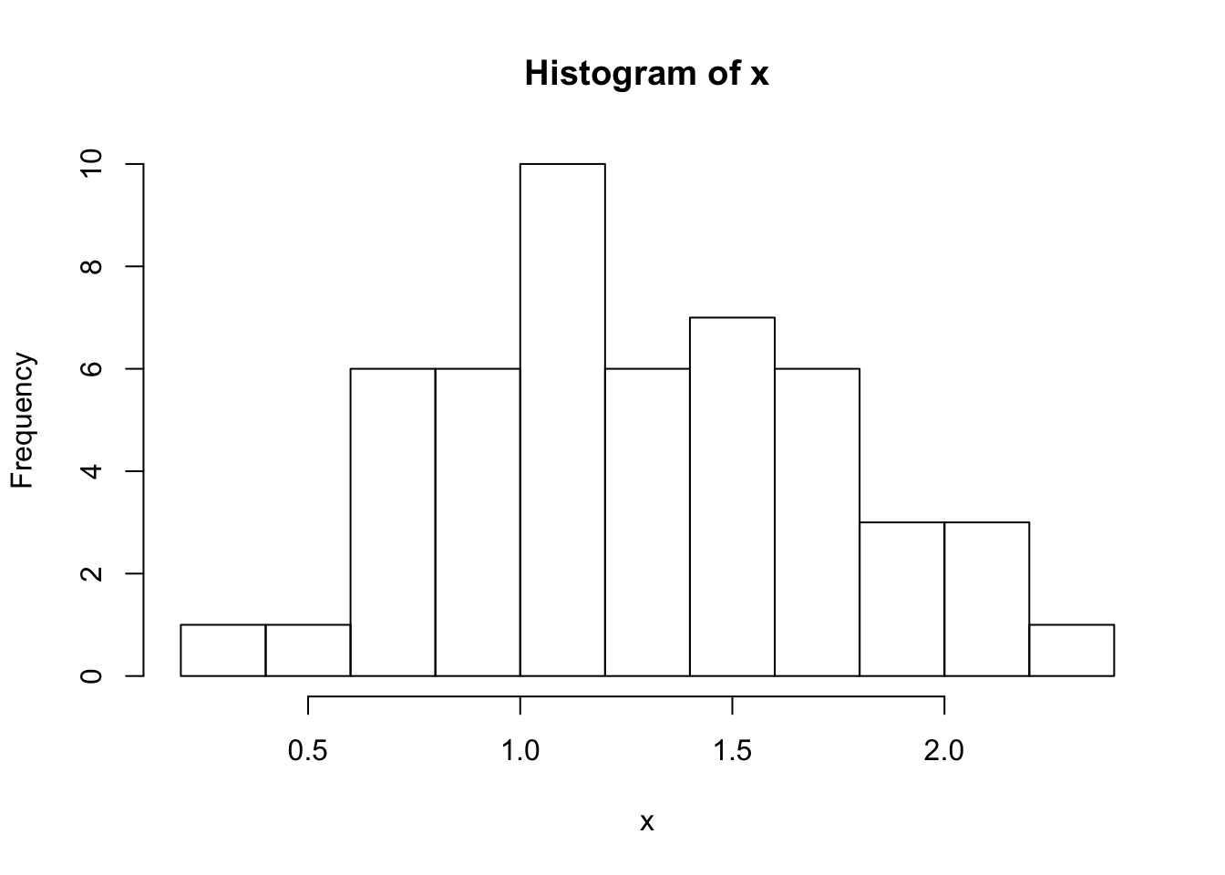

Here are the stats for our mean, calculated the old-fashioned way from an n of 50:

mean: 1.27
SE: 0.18
95% CI: [1.14, 1.40]

Now, let’s bootstrap this mean. A way to conceptualize this is to imagine re-running your 50-person experiment over and over again, except we’re not going to be drawing new subjects from the population. Instead, we’re going to draw groups of 50 subjects from our sample, but do so with replacement. This means that some subjects may show up more than once, and some may never show up at all. We’ll take the mean of each group. We’ll do this many times–here, 1000–and so we end up with a distribution of 1000 means.

For this basic procedure, we can do it in just one line:

boot <- replicate(1000, mean(sample(x, 50, replace=TRUE)))

And here’s the resulting histogram:

lb <- sort(boot)[.025*1000]
ub <- sort(boot)[.975*1000]
#Plot a histogram of the bootstrapped distribution, the
#mean, and the 95% bootstrapped CI
hist(boot, breaks=50)
abline(v=c(mean(boot), lb, ub), col=rep('red', 3), lty=c(1, 2, 2))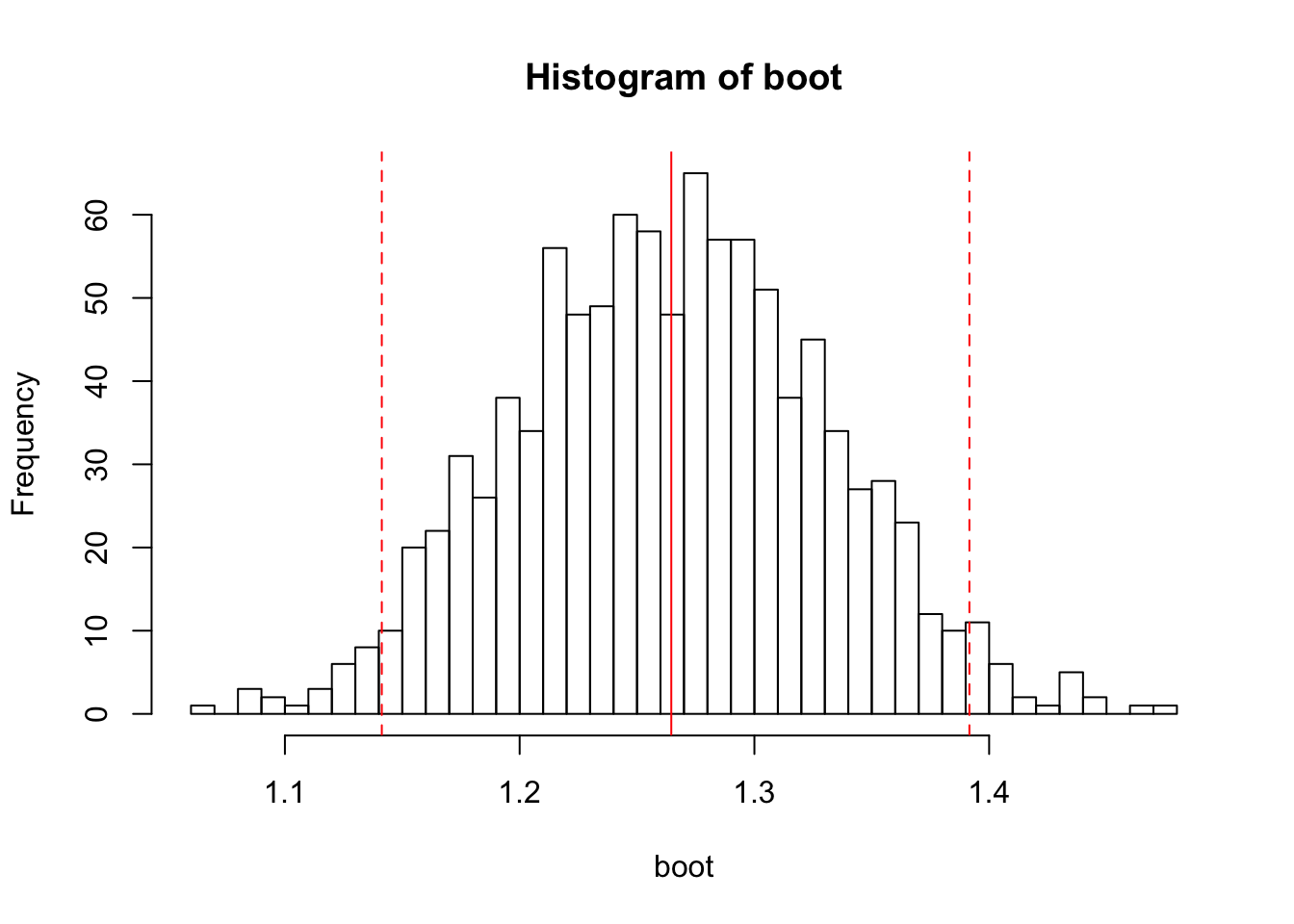

The bootstrapped mean (1.27) is of course centered on our sample mean. Now we have a distribution of values for the mean that we could expect to obtain with our sample.

Now, if we wanted to do confidence intervals, we could get the SE of the bootstrapped distribution and do it the usual way. However, we also have an option available to us called the percentile method. In order to find the confidence intervals, we sort all of our bootstrapped values, and then take the 2.5% quantile and the 97.5% quantile. If you repeat the sampling procedure with the same process on the same population (precisely what we do with our bootstrap), 95% of the time the mean falls between these endpoints. If we do this procedure with our particular sample, we get this:

95% bootstrapped CI: [1.14, 1.40]

Here, the bootstrapped CI and the standard-error derived CI match up (not that surprising, since our data is normally distributed and therefore exceptionally well-behaved!). However, if you have constrained data, such as accuracy, bootstrapped confidence intervals will automatically conform to those limits and won’t exceed 100% or dip below 0%.

Here’s an example of bootstrapping the estimate of the effect size. We’re going to assume a between-subjects design here. We’ll make two independent, normally distributed groups with a true effect of .5. I’m going to let the cohen.d function from the effsize package do the heavy lifting and give me both the estimate and the confidence interval:

groups <- data.frame('exp'=rnorm(50, .5, 1), 'control'=rnorm(50))
(es <- cohen.d(groups$exp, groups$control))

## 
## Cohen's d
## 
## d estimate: 0.6359746 (medium)
## 95 percent confidence interval:
##     lower     upper 
## 0.2291717 1.0427774

Here’s how we would bootstrap those same intervals. We resample each group independently, because it’s between-subjects. The procedure is much the same if it’s within subjects, except you would resample your pairs of data because the two groups are not independent in that case. The code:

boot_es <- replicate(1000, cohen.d(sample(groups$exp, 50, replace=TRUE), 
                                   sample(groups$control, 50, replace=TRUE))$estimate)

And here’s the histogram of the bootstrapped distribution, with the mean and bootstrapped CI plotted:

lb_es <- sort(boot_es)[.025*1000]
ub_es <- sort(boot_es)[.975*1000]
hist(boot_es, breaks=50)
abline(v=c(mean(boot_es), lb_es, ub_es), col=rep('red', 3), lty=c(1, 2, 2))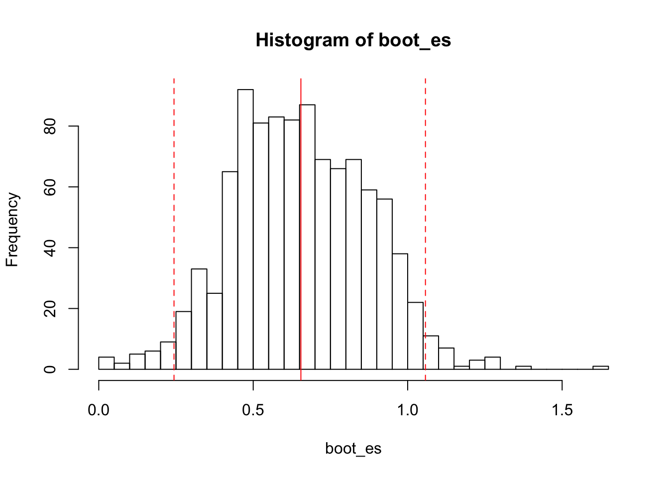

bootstrapped mean: .56
95% bootstrapped CI: [.14, .99]

And there you have it: bootstrapped confidence intervals on your effect sizes.

There is an incredible amout of nuance in the bootstrap method, and many different ways to apply it to even the most complex data. You can use it for something as simple as confidence intervals on a mean, or as complicated as regression coefficients. It’s also great for getting CI estimates for statistics or measures that don’t have a formula method. The general idea–resample your own data to get estimates–underlies even the most complex applications of this method. If you understand the basic logic, it’s pretty easy to understand and start using new applications.

If you are mathematically inclined, there have been many proofs and a lot of work showing the first- and second-order correctness of bootstrapping estimations. The method I showed here for confidence intervals is just the percentile method; although it has been shown to work well in a wide variety of situations, there are other approaches, some which offer bias correction and other improvements (for example).

If you want to get started, there are some R packages that will handle bootstrapping for you:

boot (general-purpose, and can generate many variants of the various methods)
bootES (for effect sizes in particular)

And of course, if you want a really deep dive, you can check out the original book:

Efron & Tibshirani, An Introduction to the Bootstrap. Chapman & Hall/CRC, 1993.

Comments